Diffusion models (DMs) operate through a forward process that gradually adds Gaussian noises to data, described as follows: \[ \begin{equation}z_{t} = \sqrt{{\alpha}_t} z_0 + \sqrt{1 - {\alpha}_t} \varepsilon\quad \varepsilon \sim \mathcal{N}(0,\mathcal{I}) \end{equation} \]
where \(z_0\) is a sample from the data distribution, \({\alpha}_{1:T}\) specify a variance schedule for \(t\sim [1, T]\). The training objective involves a parameterized noise prediction network, \(\varepsilon_{\theta}\), which aims to reverse the diffusion process. The training objective is to minimize the following loss based on a chosen metric function for measuring the distance between two samples \(d(\cdot, \cdot)\): \[ \begin{equation}\min_\theta \mathbb{E}_{z_0, \varepsilon, t} \big[d\left(\varepsilon, \varepsilon_{\theta}(z_t,t)\right)\big] \end{equation} \]
Sampling from a diffusion model is an iterative process that progressively denoises the data. Following Eq (12) in Song et al. (2020), the denoising step at \( t \) is formulated as: \[ \begin{equation} \begin{aligned} z_{t-1} = & \sqrt{{{\alpha}}_{t-1}} \left( \frac{z_t - \sqrt{1 - {{\alpha}}_t} \varepsilon_{\theta}(z_t, t)}{\sqrt{{\alpha}}_t} \right) \quad \text{(predicted } z_0 \text{)} \\ & + \sqrt{1 - {\alpha}_{t-1} - \sigma_t^2} \cdot \varepsilon_{\theta}(z_t,t) \quad \text{(direction to } z_t \text{)} \\ & + \sigma_t \varepsilon_t\quad \text{where } \varepsilon_t \sim \mathcal{N}(0,\mathcal{I}) \quad \text{(random noise)} \end{aligned} \end{equation} \]
DDPM sampling introduces a noise schedule \(\sigma_t\) so that Eq (3) becomes Markovian. By setting \(\sigma_t\) to vanish, DDIM sampling results in an implicit probabilistic model with a deterministic forward process.
Following DDIM, we can use the function \(f_\theta\) to predict and reconstruct \(\bar{z_0}\) given \(z_t\): \[ \begin{equation} \bar{z}_0 = f_\theta(z_t, t) = \left(z_t - \sqrt{1 - {\alpha}_t} \cdot \varepsilon_\theta(z_t, t) \right) / \sqrt{{\alpha}_t} \end{equation} \]
Recently, Latent Diffusion Models (LDMs) offer a new paradigm by operating in the latent space. The source latent \(z_0\) is acquired by encoding a sample \(x_0\) with an encoder \(\mathcal{E}\), such that \(z_0 = \mathcal{E}(x_0)\). So as to be reversed, the output can then be reconstructed by a decoder \(\mathcal{D}\). This framework presents a computationally efficient way to generate high-fidelity images, as the diffusion process is conducted in a latent space with lower dimensions.
Consistency models (CMs) have recently been introduced, which greatly accelerate the generation process compared with previous DMs. One notable property of CMs is self-consistency, such that samples along a trajectory map to the sample initial. The key is a consistency function \(f(z_t, t)\), which ensures a consistent distillation process by optimizing: \[ \begin{equation} \min_{\theta,\theta^{-};\phi} \mathbb{E}_{z_0,t} \left[d\left(f_{\theta}(z_{t_{n+1}}, t_{n+1}), f_{\theta^{-}}(\hat{z}^{\phi}_{t_{n}}, t_{n})\right)\right] \end{equation} \]
in which \(f_{\theta}\) denotes a trainable neural network that parameterizes these consistent transitions, while \(f_{\theta^{-}}\) represents a slowly updated target model used for consistency distillation, with the update rule \(\theta^- \leftarrow \mu \theta ^{-} + (1-\mu) \theta\) given a decay rate \(\mu\). The variable \(\hat{z}^\phi_{t_n}\) denotes a one-step estimation of \(z_{t_n}\) from \(z_{t_{n+1}}\).
Sampling in CMs is carried out through a sequence of timesteps \(\tau_{1:n} \in [t_0,T]\). Starting from an initial noise \(\hat{z}_T\) and \(z_0^{(T)} = f_\theta(\hat{z}_T, T)\), at each time-step \(\tau_{i}\), the process samples \(\varepsilon \sim \mathcal{N}(0, \mathcal{I})\) and iteratively updates the Multistep Consistency Sampling process: \[ \begin{equation} \begin{aligned} \hat{z}_{\tau_i} &= z_0^{(\tau_{i+1})} + \sqrt{\tau_i^2 - t_0^2 }\varepsilon \\ z_0^{(\tau_{i})} &= f_{\theta}(\hat{z}_{\tau_i}, \tau_i) \end{aligned} \end{equation} \]
Latent Consistency Models (LCMs) extend to accommodate a (text) condition \(c\), which is crucial for text-guided image manipulation. Similarly, sampling in LCMs at \(\tau_{i}\) starts with \(\varepsilon \sim \mathcal{N}(0, \mathcal{I})\) and updates:
\[ \begin{equation} \begin{aligned} \label{eq:lcm-samp} % \hat{z}_{\tau_i} &= \sqrt{{\alpha}_{\tau_i}}z_0^{(\tau_{i+1})} + \sqrt{1-{\alpha}_{\tau_i}} \varepsilon, \\ \hat{z}_{\tau_i} &= \sqrt{{\alpha}_{\tau_i}}z_0^{(\tau_{i+1})}
+ \sigma_{\tau_i} \varepsilon, \\ z_0^{(\tau_{i})} &= f_{\theta}(\hat{z}_{\tau_i}, \tau_i, c) \end{aligned} \end{equation} \]
DDIM inversion is effective for unconditional diffusion applications, but lacks consistency with additional text or image conditions. As illustrated in Figure 1a, the predicted \(\bar{z}_0'\) deviates from the original source \(z_0\), cumulatively leading to undesirable semantic changes. This substantially restricts its use in image editing driven by natural language-guided diffusion.
To address this concern, various forms of inversion-based editing methods have been proposed. The predominating approaches utilize optimization-based inversion. These methods aim to "correct" the forward latents guided by the source prompt (referred to as the source branch) by aligning them with the DDIM inversion trajectory. To tackle the efficiency bottlenecks and suboptimal consistency, very recent work has explored dual-branch inversion. These methods separate the source and target branches in the editing process: directly revert the source branch back to \(z_0\) and iteratively calibrate the trajectory of the target branch. As shown in Figure 2a, they calculate the distance between the source branch and the inversion branch (or directly sampled from q-sampling in CycleDiffusion), and calibrate the target branch with this computed distance at each \(t\).
Proposition 1 (Denoising Diffusion Consistent Models) Consider a special case of Eq (3) when \(\sigma_t\) is chosen as \(\sqrt{1 - \alpha_{t-1}}\) across all time \(t\), the forward process naturally aligns with the Multistep (Latent) Consistency Sampling.
When \(\sigma_t=\sqrt{1 - \alpha_{t-1}}\), the second term of Eq (3) vanishes: \[ \begin{equation} \begin{aligned} z_{t-1} = & \sqrt{{{\alpha}}_{t-1}} \left( \frac{z_t - \sqrt{1 - {{\alpha}}_t} \varepsilon_{\theta}(z_t, t)}{\sqrt{{\alpha}}_t} \right) && \text{(predicted $z_0$)} \\ & + \sqrt{1 - \alpha_{t-1}} \varepsilon_t\quad \varepsilon_t \sim \mathcal{N}(0,\mathcal{I}) && \text{(random noise)} \end{aligned} \end{equation} \]
Consider \(f(z_t, t; z_0) = \left( z_t - \sqrt{1 - {\alpha}_t} \varepsilon'(z_t,t;z_0) \right) / \sqrt{{\alpha}_t}\), where the initial \(z_0\) is available (which is the case for image editing applications) and we replace the parameterized noise predictor \(\varepsilon_\theta\) with \(\varepsilon'\) more generally. Eq (8) becomes \[ \begin{equation} \begin{aligned} z_{t-1} = \sqrt{{{\alpha}}_{t-1}} f(z_t,t;z_0) + \sqrt{1 - \alpha_{t-1}} \varepsilon_t \end{aligned} \end{equation} \] which is in the same form as the Multistep Latent Consistency Sampling step in Eq (7).
In order to make \(f(z_t, t)\) self-consistent so that it can be considered as a consistency function, i.e., \(f(z_t, t; z_0) = z_0\), we can directly solve the equation and \(\varepsilon'\) can be computed without parameterization: \[ \begin{equation} \varepsilon^{\text{cons}} = \varepsilon'(z_t, t;z_0) = \frac{z_t - \sqrt{{\alpha}_t} z_0}{\sqrt{1 - {\alpha}_t}} \end{equation} \]
As illustrated in Figure 1c, we arrive at a non-Markovian forward process, in which \(z_t\) directly points to the ground truth \(z_0\) without neural prediction, and \(z_{t-1}\) does not depend on the previous step \(z_t\) like a consistency model. We name this Denoising Diffusion Consistent Model (DDCM).

Figure 1. While DDIM is prone to reconstruction error and requires iterative inversion, DDCM accepts any random noise to start with. It introduces a non-Markovian forward process in which \(z_t\) directly points to the ground truth \(z_0\) without neural prediction, and \(z_{t-1}\) does not depend on the previous step \(z_t\) like a consistency model.
We note that DDCM suggests an image reconstruction model without any explicit inversion operation, diverging from conventional DDIM inversion and its optimized or calibrated variations for image editing. It achieves the best efficiency as it allows the forward process to start from any random noise and supports multi-step consistency sampling. On the other hand, it ensures exact consistency between original and reconstructed images as each step on the forward branch \(z_{t-1}\) only depends on the ground truth \(z_0\) rather than the previous step \(z_t\). Due to its inversion-free nature, we name this method Virtual Inversion. As outlined in Algorithm 1, \(z = z_0\) is ensured throughout the process without parameterization.

Existing inversion-based editing methods are limited for real-time and real-world language-driven image editing applications. First, most of them still depend on a time-consuming inversion process to obtain the inversion branch as a set of anchors. Second, consistency remains a bottleneck given the efforts from optimization and calibration. Recall that dual-branch inversion methods perform editing on the target branch by iteratively calibrating the \({z}_t^\textrm{tgt}\) with the actual distance between the source branch and the inversion branch at \(t\), as is boxed in Figure 3a. While they ensure faithful reconstruction by leaving the source branch untouched from the target branch, the calibrated \(z_t^\textrm{tgt}\) does guarantee consistency from \(z_t^\textrm{src}\) in the source branch, as can be seen from the visible difference between \({z}_0^\textrm{src}\) and \({z}_0^\textrm{tgt}\) in Figure 3a. Third, all current inversion-based methods rely on variations of diffusion sampling, which are incompatible with efficient Consistency Sampling using LCMs.
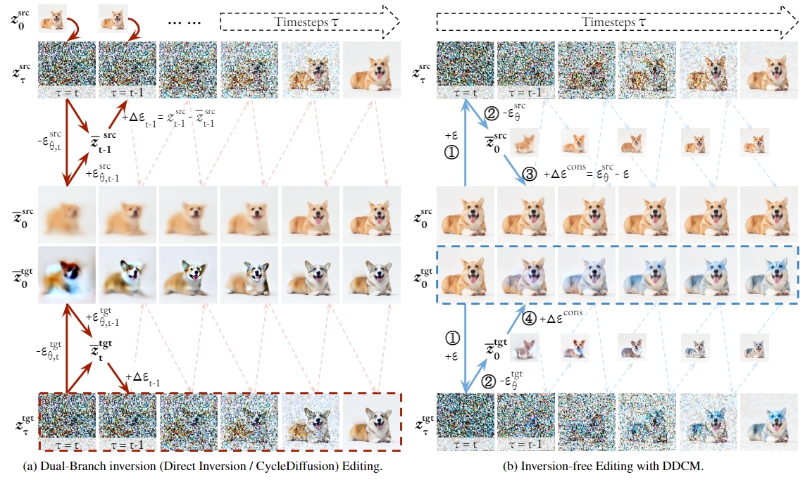
Figure 2. A comparative overview of the dual-branch inversion editing and inversion-free editing with DDCM. We initialize \(z_0^\textrm{tgt}\) with \(z_0^\textrm{src}\) in DDCM sampling for visualization purposes, while in principle it can start from any random noise. The circled numbers correspond to Algorithm 2.
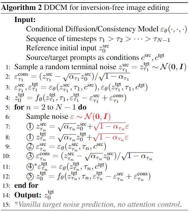
DDCM offers an alternative to address these limitations, introducing an Inversion-Free Image Editing (InfEdit) framework. While also adopting a dual-branch paradigm, the key of our InfEdit method is to directly calibrate the initial \({z}_0^\textrm{tgt}\) rather than the \({z}_t^\textrm{tgt}\) along the branch, as is boxed in Figure 3b. InfEdit starts from a random terminal noise \(z^{\textrm{src}}_{\tau_1} = z^{\textrm{tgt}}_{\tau_1} \sim \mathcal{N}(0,\mathcal{I})\). As shown in Figure 3b, the source branch follows the DDCM sampling process without explicit inversion, and we directly compute the distance \(\Delta\varepsilon^\textrm{cons}\) between \(\varepsilon^\textrm{cons}\) the \(\varepsilon_\theta^\textrm{src}\) (the predicted noise to reconstruct a \(\bar{z}_0^\textrm{src}\)). For the target branch, we first compute the \(\varepsilon_\theta^\textrm{tgt}\) to predict \(\bar{z}_0^\textrm{tgt}\), and then calibrate the predicted target initial with the same \(\Delta\varepsilon^\textrm{cons}\). Algorithm 2 outlines the mathematical details of this process, in which we slightly abuse the notation to define \(f_\theta(z_t,t,\varepsilon) = \left( z_t - \sqrt{1 - {\alpha}_t} \varepsilon \right) / \sqrt{{\alpha}_t}\).
InfEdit addresses the current limitations of inversion-based editing methods. First, DDCM sampling allows us to abandon the inversion branch anchors required by previous methods, saving a significant amount of computation. Second, the current dual-branch methods calibrate \(z_t^\textrm{tgt}\) over time, while InfEdit directly refines the predicted initial \(z_0^\textrm{tgt}\), without suffering from the cumulative errors over the course of sampling. Third, our framework is compatible with efficient Consistency Sampling using LCMs, enabling efficient sampling of the target image within very few steps.
InfEdit suggests a general inversion-free framework for image editing motivated by DDCM. In the realm of language-driven editing, achieving a nuanced understanding of the language condition and facilitating finer-grained interaction across modalities becomes a challenge. Prompt-to-Prompt noticed that the interaction between the text and image modalities occurs in the parameterized noise prediction network \(\varepsilon_\theta\), and opened up a series of attention control methods to compute a noise \(\widehat{\varepsilon_\theta^\textrm{tgt}}\) that more accurately aligns with the language prompts. In the context of InfEdit specifically, attention control refines the original predicted target noise \(\varepsilon_\theta^\textrm{tgt}\) (noted in ④ in Algorithm 2 and Figure 2b with \(\widehat{\varepsilon_\theta^\textrm{tgt}}\).
We follow Prompt-to-Prompt (P2P) in terms of notation. Each basic block of the U-Net noise predictor contains a cross-attention module and a self-attention module. The spatial features are linearly projected into queries (\(Q\)). In cross-attention, the text features are linearly projected into keys (\(K\)) and values (\(V\)). In self-attention, the keys (\(K\)) and values (\(V\)) are also obtained from linearly projected spatial features. The attention mechanism can be given as: \[ \begin{equation} \text{Attention}(K,Q,V) = MV = \textrm{softmax}\left(\frac{QK^T}{\sqrt{d}}\right)V \end{equation} \] in which \(M_{i,j}\) represents the attention map that determines the weight to aggregate the value of the \(j\)-th token on pixel \(i\), and \(d\) denotes the dimension for \(K\) and \(Q\).
Natural language specifies a wide spectrum of semantic changes. In the following, we describe how
rigid semantic changes, e.g., those on the visual features and background, can be controlled via cross attention; and
how
non-rigid semantic changes, e.g., those leading to adding/removing an object, novel action manners and physical state changes of objects, can be controlled via mutual self-attention. We then introduce a Unified
Attention Control (UAC) protocol for both types of semantic changes.
Prompt-to-Prompt (P2P) observed that cross-attention layers can capture the interaction between the spatial structures of pixels and words in the prompts, even in early steps. This finding makes it possible to control the cross-attention for editing rigid semantic changes, simply by replacing the cross-attention map of generated images with that of the original images.
Global Attention Refinement: At time step \(t\), we compute the attention map \(M_{t}\) averaged over layers given the noised latent \(z_t\) and the prompt for both source and target branch. We drop the time step for simplicity and represent the source and target attention maps as \(M^{\textrm{src}}\) and \(M^{\textrm{tgt}}\). To represent the common details, an alignment function \(A(i) = j\) is introduced which signifies that the \(i^{\textrm{th}}\) word in the target prompt corresponds to the \(j^{\textrm{th}}\) word in the source prompt. Following P2P, we refine the target attention map by injecting the source attention map over the common tokens. \[ \begin{equation} \textrm{Refine}(M^{\textrm{src}},M^{\textrm{tgt}})_{i,j} = \begin{cases} \left(M^{\textrm{tgt}}\right)_{i,j} & \text{if} A(j)=\text{None} \\ \left(M^{\textrm{src}}\right)_{i,A(j)} & \text{otherwise} \end{cases} \end{equation} \] This ensures that the common information from the source prompt is accurately transferred to the target, while the requested changes are made.
Local Attention Blends: Besides global attention refinement, we adapt the blended diffusion mechanism from Blended Diffusion and Prompt-to-Prompt (P2P). Specifically, the algorithm takes optional inputs of target blend words \(w^{\textrm{tgt}}\), which are words in the target prompt whose semantics need to be added; and source blend words \(w^{\textrm{src}}\), which are words in the source prompt whose semantics need to be preserved. At time step \(t\), we blend the noised target latent \(z_t^{\textrm{tgt}}\) following: \begin{equation} \begin{aligned} m^{\textrm{tgt}} &= \text{Threshold} \big[M_t^{\textrm{tgt}}(w^{\textrm{tgt}}), a^{\textrm{tgt}}\big] \\ m^{\textrm{src}} &= \text{Threshold} \big[M_t^{\textrm{src}}(w^{\textrm{src}}), a^{\textrm{src}}\big] \\ z_t^{\textrm{tgt}} &= (1-m^{\textrm{tgt}}+m^{\textrm{src}}) \odot z_t^{\textrm{src}} + (m^{\textrm{tgt}}-m^{\textrm{src}}) \odot z_t^{\textrm{tgt}} \\ \end{aligned} \end{equation}
in which \(m^{\textrm{tgt}}\) and \(m^{\textrm{src}}\) are binary masks obtained by calibrating the aggregated attention maps \(M_t^{\textrm{tgt}}(w^{\textrm{tgt}}),M_t^{\textrm{src}}(w^{\textrm{src}})\) with threshold parameters \(a^{\textrm{tgt}}\) and \(a^{\textrm{src}}\).
Scheduling Cross-Attention Control: Applying cross-attention control throughout the entire sampling schedule will overly focus on spatial consistency, leading to an inability to capture the intended changes. Follow P2P, we perform cross-attention control only in early steps before \(\tau_c\), interpreted as the cross-attention control strength: \[ \begin{equation} \textrm{CrossEdit}(M^{\textrm{src}},M^{\textrm{tgt}},t):=\begin{cases}\textrm{Refine}(M^{\textrm{src}},M^{\textrm{tgt}}) &t \geq \tau_c \\ M^{\textrm{tgt}} & t < \tau_c\end{cases} \end{equation} \]
One key limitation of cross-attention control lies in its inability in non-rigid editing. Instead of applying controls over the cross-attention modules, MasaCtrl observed that the layout of the objects can be roughly formed in the self-attention queries, covering the non-rigid semantic changes complying with the target prompt. The core idea is to synthesize the structural layout with the target prompt in the early steps with the original \(Q^{\textrm{tgt}}, K^{\textrm{tgt}}, V^{\textrm{tgt}}\) in the self-attention; and then to query semantically similar contents in \(K^{\textrm{src}}, V^{\textrm{src}}\) with the target query \(Q^{\textrm{tgt}}\).
Controlling Non-Rigid Semantic Changes: MasaCtrl suffers from the issue of undesirable non-rigid changes. As shown in results, MasaCtrl can lead to significant inconsistency from the source images, especially in terms of the composition of objects and when there are multiple objects and complex backgrounds. This is not surprising, as the target query \(Q^{\textrm{tgt}}\) is used throughout the self-attention control schedule. Instead of relying on the target prompts to guide the premature steps, we form the structural layout with the source self-attention \(Q^{\textrm{src}}, K^{\textrm{src}}, V^{\textrm{src}}\) in the self-attention. We show in results that this design enables high-quality non-rigid changes while maintaining satisfying structural consistency.
Scheduling Mutual Self-Attention Control: This mutual self-attention control is applied in the later steps after \(\tau_s\), interpreted as the mutual self-attention control strength: \[ \begin{equation} \begin{aligned} \textrm{SelfEdit}(\{Q^{\textrm{src}},K^{\textrm{src}},V^{\textrm{src}}\},\{Q^{\textrm{tgt}},K^{\textrm{tgt}},V^{\textrm{tgt}}\},t) := \\ \begin{cases}\{Q^{\textrm{src}},K^{\textrm{src}},V^{\textrm{src}}\}&t \geq \tau_s \\ \{Q^{\textrm{tgt}},K^{\textrm{src}},V^{\textrm{src}}\} & t < \tau_s\end{cases}\\ \end{aligned} \end{equation} \]
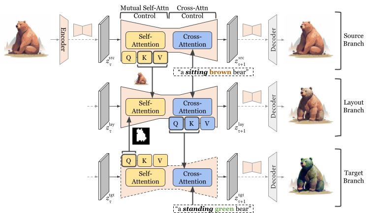
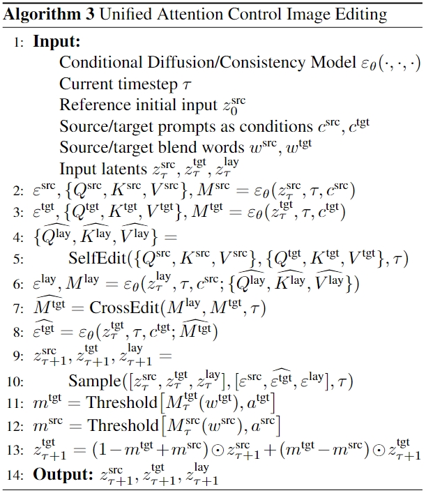
Figure 3. The proposed United Attention Control (UAC) framework to unify cross-attention control and mutual self-attention control. UAC introduces an additional layout branch as an intermediate to host the desired composition and structural information in the target image.
The UAC framework is detailed in Algorithm 3 and illustrated in Figure 3. During each forward step of the diffusion process, UAC starts with mutual self-attention control on \(z^{\textrm{src}}\) and \(z^{\textrm{tgt}}\) and assigns the output to the layout branch latent \(z^{\textrm{lay}}\). Following this, cross-attention control is applied on \(M^{\textrm{lay}}\) and \(M^{\textrm{tgt}}\) to refine the semantic information for \(M^{\textrm{tgt}}\). As is shown in Figure 3, the layout branch output \(z_0^{\textrm{lay}}\) reflects the requested non-rigid changes (e.g., "standing"), while preserving the non-rigid content semantics (e.g., ``brown''). The target branch output \(z_0^{\textrm{tgt}}\) builds upon the structural layout of the \(z_0^{\textrm{lay}}\) while reflecting the requested non-rigid changes (e.g., "green").
@article{xu2023infedit,
   title={Inversion-Free Image Editing with Natural Language},
  author={Sihan Xu and Yidong Huang and Jiayi Pan and Ziqiao Ma and Joyce Chai},
  journal={arXiv preprint arXiv:2312.04965},
  year={2023}
}